Chapter 8 Canonical transformations

8.1 Generating functionals

Under a general (invertible) transformation of the dependent variables,

\begin{equation} \label {eq:339} q'^\alpha =q'^\alpha (q,p,t),\quad p'_\alpha =p'_\alpha (q,p,t) \iff z'^A=z^A(z,t), \end{equation}

there is no guarantee that the Hamiltonian equations of motion keep, the same form, that is to say, that there exists a suitable Hamiltonian \(H'(q',p',t)\) such that the Hamiltonian equations of motion in the old variables (6.22) are equivalent to

\begin{equation} \label {eq:340} \dot q'^\alpha =\frac {\partial H'}{\partial p'_\alpha },\quad \dot p'_\alpha =-\frac {\partial H'}{\partial q^\alpha }. \end{equation}

However, if one can find a function \(G(z',t)\) such that

\begin{equation} \label {eq:341} \big [p_\alpha \dot q^\alpha -H\big ]\big |_{z(z',t)}=p'_\alpha \dot q'^\alpha -H'(z',t)+\frac {d G}{dt}, \end{equation}

then Hamilton’s equations in the new variables (8.2) are equivalent to Hamilton’s equations in the old variables (6.22).

The proof uses the fact that the addition of a total derivative does not change the equations of motion, so that the Euler-Lagrange equations of motion with respect to \(z'^A\) of the right hand side are given by (8.2). The result follows from the covariance of the Euler-Lagrange equations of motions, which guarantees that the Euler-Lagrange equations of motion of the left hand side with respect to \(z'^A\) are equivalent to the Euler Lagrange equations of \(L_H\) with respect to \(z^A\), which coincide with Hamilton’s equations (6.22).

More explicitly, in terms of equations, recall that \(L_H(z,\dot z,t)=p_\alpha \dot q^\alpha -H(z,t)\). It follows that

\begin{equation} \label {eq:372} L'_H(z',\dot z',t)=L_H\big (z(z',t),\frac {d}{dt} z(z',t),t\big )= p'_\alpha \dot q'^\alpha -H'(z',t)+\frac {d}{dt}G \end{equation}

where the first equality is the definition of the transformed first order Lagrangian, while the second equality is equivalent to the assumption (8.3).

When taking the Euler-Lagrange derivative of this equation with respect to \(z'^A\), we get on the left hand side

\begin{equation} \label {eq:373} \frac {\delta L'_H}{\delta z'^A}=\frac {\partial z^B}{\partial z'^A}\frac {\delta L_H}{\delta z^B}\Big |_{z=z(z',t)}, \end{equation}

when using covariance of the Euler-Lagrange derivatives (cf. equation (7.5)). Since Euler-Lagrange derivatives annihilate total derivatives, (4.29), the right hand side reduces to

\begin{equation} \label {eq:374} \frac {\delta }{\delta z'^A}\big [p'_\alpha \dot q'^\alpha -H'(z',t)\big ] \end{equation}

When requiring these Euler-Lagrange derivatives to vanish, one finds Hamilton’s equations of motion in the new variables, (8.2), while requiring (8.5) to vanish is equivalent to Hamilton’s equations in the old variables.

Suppose now that one may use as variables \(q^\alpha ,q'^\alpha ,t\), or in other words that \(p_\alpha =p_\alpha (q',p'(q,p,t),t)\) may be solved for \(p_\alpha \) so as to provide \(p_\alpha =p_\alpha (q,q',t)\). Let us define

\begin{equation} \label {eq:342} \Gamma _1(q,q',t)=G\Big (q',p'\big (q,p(q,q',t),t\big ),t\Big ). \end{equation}

In these variables, (8.3) becomes

\begin{equation} \begin{split} \label {eq:343} &p_\alpha (q,q',t) \dot q^\alpha -H\big (q,p(q,q',t),t\big ) \\&=p'_\alpha \big (q,p(q,q',t),t\big )\dot q'^\alpha -H'\Big ((q',p'\big (q,p(q,q',t),t\big )\Big )+\dot q^\alpha \frac {\partial \Gamma _1}{\partial q^\alpha }+\dot q'^\alpha \frac {\partial \Gamma _1}{\partial q'^\alpha }+\frac {\partial \Gamma _1}{\partial t}. \end {split} \end{equation}

By identifying the coefficents of the time derivatives, this is equivalent to

\begin{equation} \label {eq:344} \boxed {p_\alpha =\frac {\partial \Gamma _1}{\partial q^\alpha },\quad p'_\alpha =-\frac {\partial \Gamma _1}{\partial q'^\alpha }, \quad H'=H+\frac {\partial \Gamma _1}{\partial t}}. \end{equation}

The information on the canonical transformation defined by (8.3) is thus contained in the “generating function” (of the first kind) \(\Gamma _1(q,q',t)\), where one assumes that

\begin{equation} \label {eq:345} |\frac {\partial ^2 \Gamma _1}{\partial q^\alpha \partial q'^\beta }|\neq 0 \end{equation}

so that one may solve \(p_\alpha =p_\alpha (q,q',t)\) in terms of \(q'^\alpha =q'^\alpha (q,p,t)\).

In particular for instance, if \(\Gamma _1=q^\alpha \delta _{\alpha \beta }q'^\beta \), the transformation becomes \(p_\alpha =q'_\alpha \), \(p'_\alpha =-q_\alpha \), so that this transformation exchanges the role played by the generalized coordinates and the momenta,

\begin{equation} (q^\alpha ,p_\alpha )\to (p_\alpha ,-q^\alpha ).\label {eq:346} \end{equation}

In the considerations below, let us focus for notational simplicity on a single degree of freedom and omit the explicit time dependence. Consider then the (opposite of the) Legendre transform of \(\Gamma _1(q,q')\) for which \(p'=-\frac {\partial \Gamma _1}{\partial q'}\) with respect to \(q'\),

\begin{equation} \label {eq:347} \Gamma _2(q,p')=\Big [p'q'+\Gamma _1(q,q')\Big ]\Big |_{q'=q'(q,p')}. \end{equation}

This is the generating function of the second kind, for which

\begin{equation} \label {eq:348} p=\frac {\partial \Gamma _2}{\partial q},\quad q'=\frac {\partial \Gamma _2}{\partial p'}. \end{equation}

In particular, if \(\Gamma _2=qp'\), the transformation is the identity, \(p=p'\), \(q'=q\).

The Legendre transform of \(\Gamma _1\) with respect to \(q\), where \(p=\frac {\partial \Gamma _1}{\partial q}\) is the generating function of the third kind,

\begin{equation} \label {eq:349} \Gamma _3(p,q')=\Big [-pq+\Gamma _1(q,q')\Big ]\Big |_{q=q(p,q')}, \end{equation}

for which

\begin{equation} \label {eq:350} p'=-\frac {\partial \Gamma _3}{\partial q'},\quad q=-\frac {\partial \Gamma _3}{\partial p}. \end{equation}

In particular, if \(\Gamma _3=pq'\), the transformation is \(p=-p'\), \(q'=-q\).

Finally, the generating function of the fourth kind is the Legendre transform of \(\Gamma _2(q,p')\), for which \(p=\frac {\partial \Gamma _2}{\partial q}\) with respect to \(q\),

\begin{equation} \label {eq:351} \Gamma _4(p,p')=\Big [-pq+\Gamma _2(q,p')\Big ]\Big |_{q=q(p,p')}, \end{equation}

for which

\begin{equation} \label {eq:352} q'=\frac {\partial \Gamma _4}{\partial p'},\quad q=-\frac {\partial \Gamma _4}{\partial p}. \end{equation}

In particular, if \(\Gamma _4=pp'\), \(q'=p\), \(q=-p'\).

Remark: For several canonical pairs, one may have generating functions of different type in the different canonical pairs.

How can one remember these formulas ?

\begin{equation} \label {eq:353} q,q':\ pdq=p'dq'+d\Gamma _1(q,q'),\ \boxed {p=\frac {\partial \Gamma _1}{\partial q},\ p'=-\frac {\partial \Gamma _1}{\partial q'}}, \end{equation}

\begin{equation} \label {eq:354} \begin{split} q,p':\ p'dq'=d(p'q')-dp'q',\ \Gamma _2=\Gamma _1+p'q',\\ pdq=-dp'q'+d\Gamma _2(q,p'),\ \boxed {p=\frac {\partial \Gamma _2}{\partial q},\ q'=\frac {\partial \Gamma _2}{\partial p'}}, \end {split} \end{equation}

\begin{equation} \label {eq:355} \begin{split} p,q':\ pdq=d(pq)-dpq,\ \Gamma _3=\Gamma _1-pq,\\ -dpq=p'dq'+d\Gamma _3(p,q'),\ \boxed {q=-\frac {\partial \Gamma _3}{\partial p},\ p'=-\frac {\partial \Gamma _3}{\partial q'}}, \end {split} \end{equation}

\begin{equation} \label {eq:356} \begin{split} p,p':\ \Gamma _4=\Gamma _2-pq=\Gamma _3+p'q',\\ -dpq=-dp'q'+d\Gamma _4(p,p'),\ \boxed {q=-\frac {\partial \Gamma _4}{\partial p},\, q'=\frac {\partial \Gamma _4}{\partial p'}}. \end {split} \end{equation}

Remark: The transformation

\begin{equation} q'=\mu q,\quad p'=\nu p,\quad \mu ,\nu \in \mathbb R^*, \label {eq:357} \end{equation}

is a canonical transformation with

\begin{equation} \label {eq:358} H'(q',p',)=\mu \nu H(\frac {q'}{\mu },\frac {p'}{\nu }) \end{equation}

because

\begin{equation} \label {eq:359} p'\dot q'-H'=\mu \nu \big (p\dot q-H\big )\big |_{q=\frac {q'}{\mu },p=\frac {p'}{\nu }}, \end{equation}

and the Euler-Lagrange equations are unchanged when multiplying the Lagrangian by a non-vanishing constant. There exists no generating function however. The same holds for the canonical transformation

\begin{equation} \label {eq:360} q'=p,\quad p'=q,\quad H'=-H. \end{equation}

A canonical transformation that admits a generating function is called a restricted canonical transformation.

8.2 Invariance of canonical Poisson brackets

Remarks:

(i) The last condition becomes explicitly

\begin{equation} \label {eq:362} \frac {\partial z'^A}{\partial z^C}\omega ^{CD}\frac {\partial z'^B}{\partial z^D}=\omega ^{AB}\iff \frac {\partial z'^A}{\partial z^C}\omega ^{CD}= \omega ^{AB}\frac {\partial z^D}{\partial z'^B}, \end{equation}

or

\begin{equation} \label {eq:363} \begin{pmatrix} \frac {\partial q'^\alpha }{\partial q^\beta } & \frac {\partial q'^\alpha }{\partial p_\beta } \\ \frac {\partial p'_\alpha }{\partial q^\beta } & \frac {\partial p'_\alpha }{\partial p_\beta } \end {pmatrix}\begin{pmatrix} 0 & \delta ^\beta _\gamma \\ -\delta ^\gamma _\beta & 0 \end {pmatrix}=\begin{pmatrix} 0 & \delta ^\alpha _\beta \\ -\delta ^\beta _\alpha & 0 \end {pmatrix}\begin{pmatrix} \frac {\partial q^\gamma }{\partial q'^\beta } & \frac {\partial p_\gamma }{\partial q'^\beta } \\ \frac {\partial q^\gamma }{\partial p'_\beta } & \frac {\partial p_\gamma }{\partial p'_\beta } \end {pmatrix}, \end{equation}

which is equivalent to the following relations between mixed partial derivatives:

\begin{equation} \label {eq:364} \begin{split} \frac {\partial q'^\alpha }{\partial p_\gamma }=-\frac {\partial q^\gamma }{\partial p'_\alpha }\ (a),\quad \frac {\partial q'^\alpha }{\partial q^\gamma }=-\frac {\partial p_\gamma }{\partial p'_\alpha }\ (b),\\ \frac {\partial p'_\alpha }{\partial p_\gamma }=-\frac {\partial q^\gamma }{\partial q'^\alpha }\ (c),\quad \frac {\partial p'_\alpha }{\partial q^\gamma }=-\frac {\partial p_\gamma }{\partial q'^\alpha }\ (d). \end {split} \end{equation}

(ii) As a consequence of the theorem, for a restricted canonical transformation, Poisson brackets can be computed in the old or in the new variables. Indeed, if \(F'(z')=F(z(z'))\), \(G'(z')=G(z(z'))\),

\begin{equation} \begin{split} \label {eq:365} \{F',G'\}_{z'}&=\frac {\partial F'}{\partial z'^A}\omega ^{AB}\frac {\partial G'}{\partial z'^B}=\frac {\partial F}{\partial z^C}\Big |_{z=z(z')}\frac {\partial z^C}{\partial z'^A}\omega ^{AB}\frac {\partial z^D}{\partial z'^B}\frac {\partial G}{\partial z^D}\Big |_{z=z(z')}\\&=\Big (\frac {\partial F}{\partial z^C}\omega ^{CD}\frac {\partial G}{\partial z^D}\Big )\Big |_{z=z(z')}=\Big (\{F,G\}\Big )\Big |_{z=z(z')}, \end {split} \end{equation}

where we have used that, by multiplying by the Jacobian matrices of the inverse transformations, the first of (8.27) is equivalent to

\begin{equation} \label {eq:366} \frac {\partial z^C}{\partial z'^A}\omega ^{AB}\frac {\partial z^D}{\partial z'^B}=\omega ^{CD}. \end{equation}

(iii) Equation (8.31) means that the inverse of a canonical transformation is a canonical transformation. Consider then also a second canonical transformations, \(z''=z''(z')\). The Jacobian matrices of the composed transformation \(z''=z''(z)=z''(z'(z))\) are given by

\begin{equation} \label {eq:367} \frac {\partial z''^A}{\partial z^B}=\frac {\partial z''^A}{\partial z'^C}\Big |_{z'=z'(z)}\frac {\partial z'^C}{\partial z^B}, \end{equation}

which allows to prove directly that the composition of two canonical transformations is a canonical transformation. This implies that canonical transformations form a (sub-) group (of the group of invertible transformations).

The detailed proof of the theorem is omitted here and can be found in the handwritten “french” notes.

In the following, we only consider restricted canonical transformations but omit the adjective “restricted”.

8.3 Infinitesimal canonical transformations

In order to study an infinitesimal canonical transformation close to the identity, we start from a generating function of the second kind of the form

\begin{equation} \label {eq:368} \Gamma _2=p'_\beta q^\beta +\epsilon G(q,p',t), \end{equation}

because we have already seen that for \(\epsilon =0\), such a canonical transformation reduces to the identity. For \(\epsilon \neq 0\), the associated canonical transformation is defined by

\begin{equation} \label {eq:369}p_\alpha =\frac {\partial \Gamma _2}{\partial q^\alpha }=p'_\alpha +\epsilon \frac {\partial G}{\partial q^\alpha },\quad q'^\alpha =\frac {\partial \Gamma _2}{\partial p'_\alpha }=q^\alpha +\epsilon \frac {\partial G}{\partial p'_\alpha }. \end{equation}

In the second terms of these relations one may replace \(p'_\beta \) by \(p_\beta \) in \(G\), since one is already at first order on \(\epsilon \), so that \(G=G(q,p,t)\). One may then write,

\begin{equation} \label {eq:370} \delta q^\alpha = q'^\alpha -q^\alpha =\epsilon \frac {\partial G}{\partial p_\alpha }=\epsilon \{q^\alpha ,G\},\quad \delta p_\alpha = p'_\alpha -p^\alpha =-\epsilon \frac {\partial G}{\partial q^\alpha }=\epsilon \{p_\alpha ,G\}, \end{equation}

and thus also

\begin{equation} \label {eq:371} \boxed {\delta z^A=\epsilon \{z^A,G\}}. \end{equation}

The phase space function \(G(q,p,t)\) is called the generator of the infinitesimal canonical transformation.

8.4 One-parameter group of canonical transformations

A family of canonical transformation depending on a parameter \(\lambda \),

\begin{equation} \label {eq:375} z_\lambda ^A=Z^A(z,\lambda ), \end{equation}

such that

\begin{equation} \label {eq:376} z^A_{\lambda _1+\lambda _2}=Z^A(z,\lambda _1+\lambda _2)= Z^A\big (Z(z,\lambda _1),\lambda _2\big ),\quad z^A_0=Z^A(z,0)=z^A, \end{equation}

is called a one-parameter group of canonical transformations.

The transformation \(z^A_{\lambda +\epsilon }\) with \(\epsilon \) infinitesimal is an infinitesimal canonical transformation that reduces to \(z^A_\lambda \) for \(\epsilon =0\). It follows from (8.36) that there exists a generator \(G(z_\lambda )\) such that

\begin{equation} \label {eq:377} z^A_{\lambda +\epsilon }-z^A_\lambda =\epsilon \{z^A_\lambda ,G(z_\lambda )\}_{z_\lambda }. \end{equation}

This can also be written as

\begin{equation} \label {eq:378} \boxed {\frac {d}{d\lambda } z^A_\lambda =-\{G(z_\lambda ),z^A_\lambda \}_{z_\lambda }}, \end{equation}

or, when using the property that Poisson brackets can be evaluated before or after a canonical transformation,

\begin{equation} \label {eq:379} \frac {d}{d\lambda }Z^A(z,\lambda )=-\{G(Z(z,\lambda )),Z^A(z,\lambda )\}_z. \end{equation}

Conversely, this equation determines uniquely a one-parameter group of canonical transformations close to the identity.

For all functions \(F(z_\lambda )\) that do not depend explicitly on \(\lambda \),

\begin{equation} \label {eq:380} \frac {d F}{d\lambda }=\frac {\partial F}{\partial z^A_\lambda }\frac {d z^A_\lambda }{d\lambda }=-\{G(z_\lambda ),z^A_\lambda \}\frac {\partial F}{\partial z^A_\lambda }=-\{G(z_\lambda ),F(z_\lambda )\}_{z_\lambda }. \end{equation}

This implies in particular that \(\frac {d G(z_\lambda )}{d\lambda }=0\) if \(\frac {\partial G}{\partial \lambda }=0\). Assuming that \(G(z_\lambda )\) has no explicit \(\lambda \) dependence thus implies that

\begin{equation} \label {eq:381} \frac {d^2 z^A_\lambda }{(d\lambda )^2}=\{G(z_\lambda ),\{G(z_\lambda ), z^A_\lambda \}_{z_\lambda }\}_{z_\lambda }, \end{equation}

and, by iteration, that

\begin{equation} \label {eq:382} \frac {d^n z^A_\lambda }{(d\lambda )^n} =(-1)^n\{G(z_\lambda ),\{G(z_\lambda ),\dots , \{G(z_\lambda ),z^A_\lambda \}_{z_\lambda }\}_{z_\lambda }\}_{z_\lambda }, \end{equation}

with \(n\) brackets. When using that \(z^A_0=z^A\) and by putting \(\lambda \) to zero, this gives

\begin{equation} \label {eq:385} \frac {d^n z^A_\lambda }{(d\lambda )^n}\Big |_{\lambda =0} =(-1)^n\{G(z),\{G(z),\dots , \{G(z),z^A\}\}\}. \end{equation}

One then may write the function in a neighborhood of the identity in terms of its Taylor series as

\begin{equation} \label {eq:386} z^A_\lambda =z^A+\sum _{n=1}\frac {(-1)^n\lambda ^n}{n!}\{G(z),\{G(z),\dots , \{G(z),z^A\}\}\}. \end{equation}

This Taylor series may also be written as

\begin{equation} \label {eq:383} {z^A_\lambda =e^{-\lambda \{G,\cdot \}} z^A=e^{-\lambda v_G}z^A}. \end{equation}

Remarks:

(i) When the generator of a one-parameter group of canonical transformations depends explicitly on the parameter \(\lambda \), it remains true that the one-parameter group is uniquely determined by the generator in a neighborhood of the identity. The explicit formula is however more involved than the exponential series above.

(ii) Given initial conditions \(z_0^A=z^A\), the solution to the equations of motion \(z^A_t=z^A(z_0,t)\) is a one-parameter group of canonical transformations whose generator is the Hamiltonian. This follows from the fact that, when \(\lambda =t\) and \(G=H\), the equations (8.40) coincide with Hamilton’s equations of motion. Furthermore, if \(H\) does not explicitly depend on time, \(\frac {\partial H}{\partial t}=0\), the solution of the equations of motion may be written as

\begin{equation} z_t=e^{-t\{H,\cdot \}}z\label {eq:387}, \end{equation}

in a neighborhood of the identity.

(iii) If \(K(z)\) is a first integral that does not depend explicitly on time, \(\{K,H\}=0\), it follows that \(K(z_t)=K(z_0)\). Indeed, \(\frac {d K(z_t)}{dt}=\{K(z_t),H(z_t)\}_{z_t}=0\).

(iv) Conversely, when considering the one-parameter group of canonical transformations \(z^A_\lambda \) generated by the first integral \(K(z)\) which does not depend explicitly on time, for a Hamiltonian that does not explicitly on \(\lambda \), it follows that \(H(z_\lambda ,t)=H(z_0,t)\) since \(\frac {d H(z_\lambda ,t)}{d \lambda }=-\{K(z_\lambda ),H(z_\lambda ,t)\}_{z_\lambda }=0\) so that \(H(z_\lambda ,t)=H(z_0,t)\).

The general case when the generator depends explicitly on the parameter can be found in the handwritten “french” notes.

8.5 Liouville theorem

For a system of first order differential equations,

\begin{equation} \label {eq:388} \dot x^a=v^a(x^b,t),\quad a,b=1,\dots ,n, \end{equation}

there is existence and uniqueness for the solution of the inital value problem,

\begin{equation} \label {eq:389} x^a_t=X^a(t;x_0^b,t_0),\quad X^a(t_0;x_0^b,t_0)=x^a_0, \end{equation}

under suitable conditions which we assume to be satisfied.

One may also interpret this equation as (time dependent) transformations that map the points with coordinates \(x^a_0\) to the points with coordinates \(x^a_t\). This group of transformation is also called a “flow”, in analogy with fluid mechanics.

Consider then a function \(\rho (x^a,t)\) and its integral over a domain \(\mathcal {D}(t)\) of \(\mathbb R^n\),

\begin{equation} \label {eq:390} I(t)=\int _{\mathcal {D}(t)}\rho (x,t) dx^1\dots dx^n. \end{equation}

When using the flow, to each point of the domain \(\mathcal {D}(t)\) corresponds a single point at a time \(t'\). This defines the domain \(\mathcal {D}(t')\).

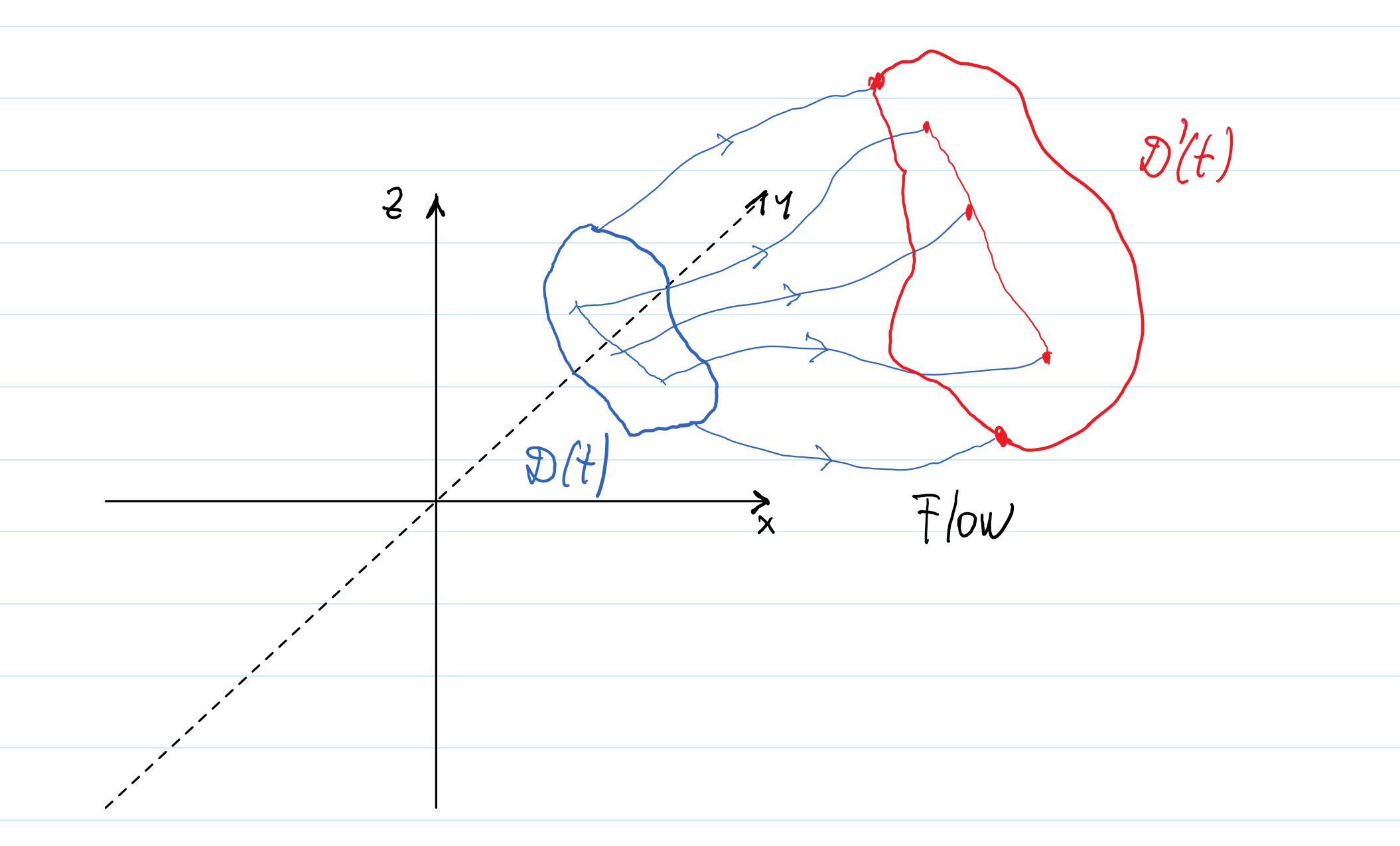
One wants to understand how the integral changes in time,

\begin{equation} \label {eq:391} I(t')-I(t)=\int _{\mathcal {D}(t')}\rho (x,t') dx^1\dots dx^n-\int _{\mathcal {D}(t)}\rho (x,t) dx^1\dots dx^n. \end{equation}

In order to do so, one uses that

\begin{equation} \int _{\mathcal {D}(t')}\rho (x,t') dx^1\dots dx^n=\int _{\mathcal {D}(t)}\rho \big (X(t';x,t),t'\big )\Big |\frac {\partial X^a}{\partial x^b}\Big |dx^1\dots dx^n,\label {eq:392} \end{equation}

to bring back the integral over the new domain to an integral over the old domain.

To see that this is indeed the case, take an example in \(1\) dimension. Remember that for a definite integral,

\begin{equation} I=\int _{x=a}^{x=b} f(x) dx,\label {eq:397} \end{equation}

if one makes a change of variables, \(x=g(y)\), the integral becomes

\begin{equation} I=\int ^{y=g^{-1}(b)}_{y=g^{-1}(a)} f(g(y))\frac {dg}{dy}dy.\label {eq:398} \end{equation}

Take the domain at time \(\mathcal {D}(t)\) to be the set of points that belong to the interval \([a,b]\), \(x_t\in [a,b]\) and

\begin{equation} \label {eq:393} I(t)=\int ^{x=b}_{x=a}\rho (x,t) dx. \end{equation}

Under the map \(x_{t'}=X(t';x,t)\), the end-point of the new domain \(\mathcal {D}(t')\) are \(X(t';a,t)\) and \(X(t';b,t)\), the images of \(x_t=a\) and \(x_t=b\). It follows that

\begin{equation} \label {eq:394} I(t')=\int ^{x=X(t';b,t)}_{x=X(t';a,t)}\rho (x,t')dx. \end{equation}

When doing the change of variables \(x=X(t';y,t)\) it follows that

\begin{equation} \label {eq:395} I(t')=\int ^{y=X^{-1}(t';X(t';b,t),t)=b}_{y=X^{-1}(t';X(t';a,t),t)=a}\rho \big (X(t';y,t),t'\big )\frac {\partial X}{\partial y}dy=\int ^{x=b}_{x=a}\rho \big (X(t';x,t),t'\big )\frac {\partial X}{\partial x}dx, \end{equation}

and thus, by generalizing to multiple variables and integrals,

\begin{equation} \label {eq:396} \boxed {I(t')-I(t)=\int _{\mathcal {D}(t)}\Big [\rho \big (X^a(t';x,t),t'\big )\Big |\frac {\partial X^a}{\partial x^b}\Big |-\rho (x,t)\Big ]dx^1\dots dx^n}. \end{equation}

In particular, it follows that \(I(t')=I(t)\) if \(\rho \) is constant and the Jacobian unity, \(|\partial X/\partial x|=1\). If \(\rho =1\), \(I(t)\) represents the volume of \(\mathcal {D}(t)\) which remains constant for a flow with unit Jacobian.

Consider transformations on phase space, so that the coordinates \(x^a\) are now the coordinates \(z^A\). For a canonical transformation, we have

\begin{equation} \label {eq:399} \frac {\partial z'^A}{\partial z^C}\omega ^{CD}\frac {\partial z'^B}{\partial z^D}=\omega ^{AB} \iff J\omega J^T=\omega ,\quad {J^A}_B=\frac {\partial z'^A}{\partial z^B}, \end{equation}

it follows that \({\rm det}\, J=\pm 1\) since \({\rm det}\,\omega =1\neq 0\). For all canonical transformations connected to the identity, one thus has by continuity that \({\rm det}\, J=1\). (One may show further that this is the case for all canonical transformations.) Since the Hamiltonian evolution is a one-parameter group of canonical transformations, with unit Jacobian, we have:

Let us now analyse the consequence of (8.59) for an infinitesimal flow, \(t'=t+\epsilon \). In this case,

\begin{equation} \label {eq:400} X^a(t+\epsilon ;x^b,t)=x^a+\epsilon v^a(x^b,t)+\mathcal {O}(\epsilon ^2), \end{equation}

while

\begin{equation} \label {eq:401} \Big |\frac {\partial X^a}{\partial x^b}\Big |=\Big |\delta ^a_b+\epsilon \frac {\partial v^a}{\partial x^b}+\mathcal O(\epsilon ^2)|=1+\epsilon \frac {\partial v^a}{\partial x^a}+\mathcal O(\epsilon ^2). \end{equation}

As a consequence,

\begin{equation} \label {eq:402} \frac {dI(t)}{dt}=\lim _{\epsilon \to 0}\frac {I(t+\epsilon )-I(t)}{\epsilon } =\int _{\mathcal D(t)}\Big [\frac {\partial \rho }{\partial t}+\frac {\partial \rho }{\partial x^a}v^a+\rho \frac {\partial v^a}{\partial x^a}] dx^1\dots dx^n. \end{equation}

It follows that

\begin{equation} \label {eq:403} \frac {d I(t)}{dt}=0,\ \forall \mathcal D(t) \iff \frac {\partial \rho }{\partial t} + \frac {\partial }{\partial x^a}(\rho v^a)=0. \end{equation}

The equation for \(\rho \) on the right hand side is called a “continuity equation”.

For a Hamiltonian system, we have \(\rho =\rho (z,t)\), while \(v^a\to \omega ^{AB}\frac {\partial H}{\partial z^B}\), and the continuity equation becomes

\begin{equation} \label {eq:404} \frac {\partial \rho }{\partial t} + \frac {\partial }{\partial z^A}(\rho \omega ^{AB}\frac {\partial H}{\partial z^B})=0\iff \boxed {\frac {\partial \rho }{\partial t}+\{\rho , H\}=0}. \end{equation}

This is the Liouville equation in statistical mechanics, for which \(\rho =1\) is a particular solution.