Chapter 6 Hamiltonian formalism

In the regular case, the Euler-Lagrange equations are equivalent to a system of \(n\) second order equations

\begin{equation} \label {eq:93} \ddot q^{\alpha }=f^{\alpha }(q^{\beta },\dot q^{\beta },t). \end{equation}

These equations may be turned into an equivalent system of \(2n\) first order differential equations by introducing additional variables \(v^{\alpha }\) and writing,

\begin{equation} \label {eq:189} \dot q^{\alpha }=v^{\alpha },\quad \dot v^{\alpha }=f^{\alpha }(q^{\beta },v^{\beta },t). \end{equation}

This system does not in general derive from a variational principle. One of the aims of the Hamiltonian formulation is to construct an equivalent system of \(2n\) first order differential equations that does follow from a variational principle. This will be done through a suitable Legendre transform below.

6.1 Legendre transform

Take a function of one variable,

\begin{equation} \label {eq:265} y=y(x), \end{equation}

and suppose that one is interested in the extrema of this function, i.e., the points \(\bar x\) such that \(y'(\bar x)=0\). The problem that one would like to address is to represent this function by using the derivative

\begin{equation} \label {eq:290} p=\frac {d y}{dx}, \end{equation}

as the dependent variable without loosing any information. Note that at each point \(x\), the derivative represents the slope of the tangent to the curve at that point, \(\frac {dy}{dx}=\tan \theta \), with \(\theta \) the angle of the tangent and the horizontal axis.

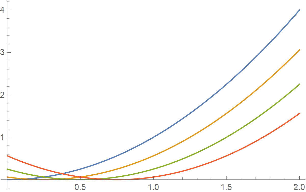
One possibility would be to invert the last equation to get \(x=x(p)\), which is possible locally when \(\frac {d^2 y}{dx^2}\neq 0\), and then to substitute into (6.3). If the original function was \(y=x^2\), one gets \(p=2x\), \(x=\frac 12 p\) and then \(y=\frac 14 p^2\). The problem is however that the relation

\begin{equation} \label {eq:291} y=\frac 14 (\frac {d y}{dx})^2, \end{equation}

does not allow one to uniquely reconstruct the parabola, with its extremum at \(\bar x=0\) Indeed, separation of variables gives

\begin{equation} \label {eq:292} \frac {dy}{2\sqrt {y}}=dx \longrightarrow \sqrt y=x-c \longrightarrow y=(x-c)^2, \end{equation}

and the original parabola is not uniquely reconstructed.

A better solution consists in representing the original curve \(y=y(x)\) by the family of tangent lines at each point. In order to do so, one represents each member of this family by two numbers \((p,\Psi )\), the slope of the tangent \(p\) and the \(-\Psi \), the intersection of the tangent line to the curve at the point \(x\) with the \(y\) axis. One then replaces the relation \(y=y(x)\) by \(\psi =\psi (p)\). In terms of equations, this means that

\begin{equation} \label {eq:293} p=\frac {\Delta y}{\Delta x}=\frac {y+\Psi }{x-0}\iff \Psi =px -y. \end{equation}

More precisely, given \(y=y(x)\), define

\begin{equation} \boxed {p=\frac {dy}{dx}}\label {eq:310}. \end{equation}

This relation can be inverted if \(\frac {d^2y}{dx^2}\neq 0\) which we assume to be the case below. Inverting gives \(x=x(p)\), and in particular also that

\begin{equation} \label {eq:309} \frac {dy}{dx}\Big |_{x(p)}=p. \end{equation}

The Legendre transform \(\Psi (p)\) is defined as

\begin{equation} \label {eq:294} \boxed {\Psi (p)=\big [px-y(x)\Big ]|_{x=x(p)}=px(p)-y(x(p))}. \end{equation}

In the particular case where \(y=x^2\), \(p=2x\), \(x=\frac 12 p\), \(\Psi (p)=\frac 1 4 p^2\).

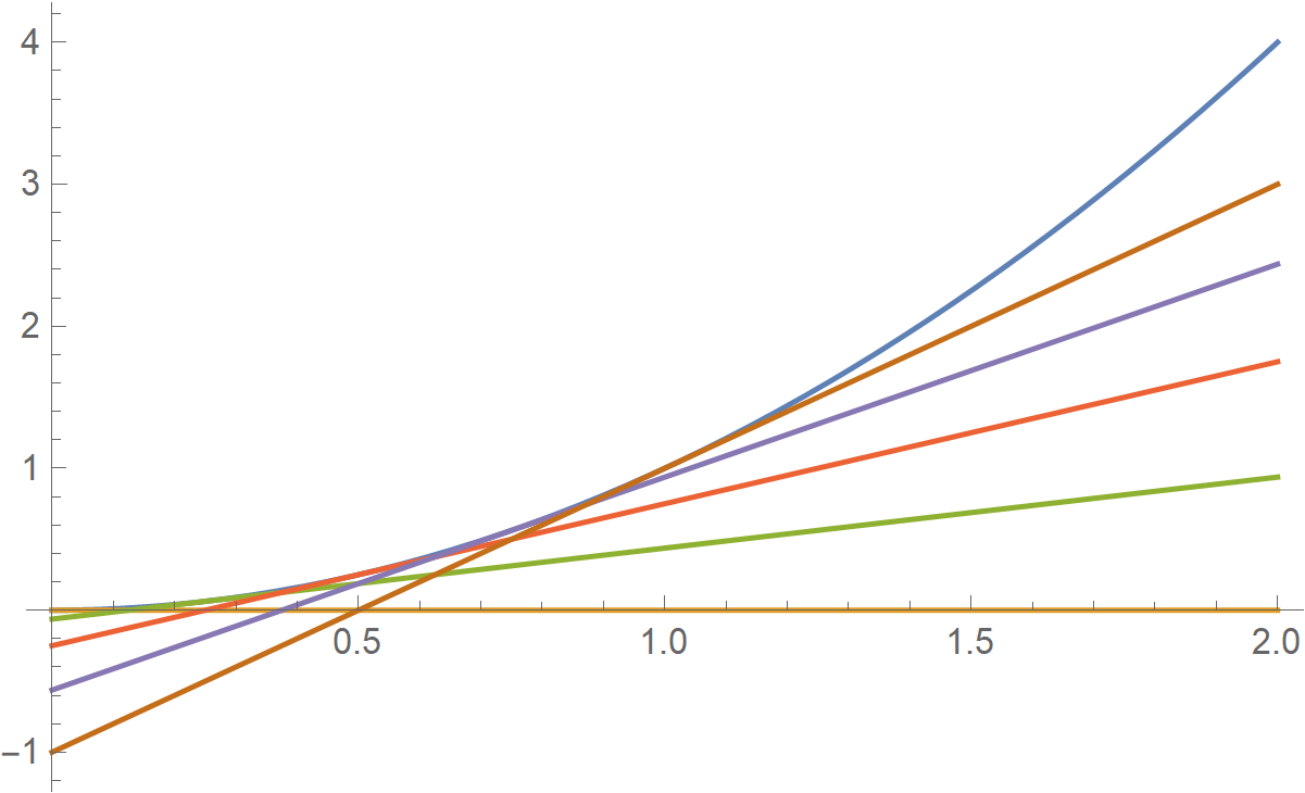
Indeed, we have to define \(\tilde x=\frac {d\Psi }{dp}\) and invert this relation to get \(p=p(\tilde x)\) and then define \(\tilde y(\tilde x)=[\tilde xp-\Psi (p)]|_{p(\tilde x)}\). When using the definition of \(\Psi \),

\begin{equation} \label {eq:295} \tilde x(p)=\frac {d}{dp}[px(p)-y(x(p))]=x(p)+\cancel {p\frac {dx}{dp}} -\cancel {\frac {dy}{dx}\Big |_{x(p)}\frac {dx}{dp}}. \end{equation}

It follows that \(\tilde x=x\) and that

\begin{equation} x=\frac {d\Psi }{dp} \label {eq:311} \end{equation}

is the inverse relation to \(p=\frac {dy}{dx}\). Furthermore,

\begin{equation} \label {eq:296} \tilde y(x)=\Big [xp-[px-y(x)]|_{x(p)}\Big ]\Big |_{p(x)}=\cancel {xp(x)} -\cancel {p(x)x}+y(x). \end{equation}

In the particular case where \(\Psi (p)=\frac 14 p^2\), \(x=\frac {\partial \Psi }{\partial p}=\frac 12 p\) so that \(p=2x\) and \(y=[xp-\frac 14 p^2]|_{p=2x}=x^2\).

The Legendre transform may be generalized to a function of several variables where some variables are transformed and others remain passive. It has important applications for instance in the context of thermodynamics.

6.2 Legendre transform in mechanics and Hamilton’s equations

Consider a Lagrangian, \(L(q^\alpha ,\dot q^\alpha ,t)\), \(\alpha =1,\dots ,n\). By definition, the Hamiltonian is the Legendre transform of the Lagrangian with respect to all the generalized velocities \(\dot q^\alpha \). One thus defines the canonical momenta by

\begin{equation} \label {eq:297} \boxed {p_\alpha =\frac {\partial L}{\partial \dot q^\alpha }}. \end{equation}

In order to be able to invert this relation,

\begin{equation} \label {eq:299} \dot q^\alpha =\dot q^{\alpha }(q^\beta ,p_\beta ,t), \end{equation}

one needs

\begin{equation} \label {eq:298} |\frac {\partial ^2 L}{\partial \dot q^\alpha \partial \dot q^\beta }|\neq 0, \end{equation}

and the Hamiltonian is

\begin{equation} \label {eq:300} \boxed {H(q^\beta ,p_\beta ,t)=\Big [p_\alpha \dot q^\alpha -L\Big ]\Big |_{\dot q^{\alpha }(q^\beta ,p_\beta ,t)}}. \end{equation}

By the theorem on the inverse Legendre transform, we thus have that

\begin{equation} \label {eq:301} \dot q^\alpha =\frac {\partial H}{\partial p_\alpha } \end{equation}

is the inverse of relation (6.14) and that

\begin{equation} \label {eq:302} L(q^\alpha ,\dot q^\alpha ,t)=\Big [p_\alpha \dot q^\alpha -H(q^\beta ,p_\beta ,t)\Big ]\Big |_{p(q,\dot q,t)}. \end{equation}

This suggests to study the least action principle based on

\begin{equation} \label {eq:303} S_H[q,p]=\int ^{t_f}_{t_i}dt\, L_H,\quad L_H=p_\alpha \dot q^\alpha -H(q^\beta ,p_\beta ,t), \end{equation}

which is first order in time derivatives. For infinitesimal virtual instantaneous variations \(\delta q^\alpha (t),\delta p_\alpha (t)\) such that \(\delta q^\alpha (t_f)=0=\delta q^\alpha (t_i)\), one finds

\begin{equation} \label {eq:304} \delta S_H=\int ^{t_f}_{t_i}dt\, [\delta p_\alpha (\dot q^\alpha -\frac {\partial H}{\partial p_\alpha })+\frac {d}{dt}(p_\alpha \delta q^\alpha )+(-\dot p_\alpha -\frac {\partial H}{\partial q^\alpha })\delta q^\alpha ], \end{equation}

so that the equations of motion that one obtains when requiring that the first order action principle be an extremum for all such variations are Hamilton’s equations

\begin{equation} \label {eq:305} \boxed { \dot q^\alpha =\frac {\partial H}{\partial p_\alpha },\quad \dot p_\alpha =-\frac {\partial H}{\partial q^\alpha }}. \end{equation}

These \(2n\) first order differential equations appear here as the Euler-Lagrange equations of \(L_H\) with respect to \(p_\alpha ,q^\alpha \).

The proof proceeds as follows. From the definition of the Legendre transform, a general variation of the Hamiltonian \(dH\) is given by

\begin{multline} \label {eq:306} \frac {\partial H}{\partial q^\alpha }dq^\alpha +\frac {\partial H}{\partial p_\alpha }dp_\alpha +\frac {\partial H}{\partial t}dt =d\Big \{\big [p_\alpha \dot q^\alpha -L(q,\dot q,t)\big ]\big |_{\dot q(q,p,t)}\Big \}\\=dp_\alpha \dot q^\alpha |_{\dot q(q,p,t)}+p_\alpha (\cancel {\frac {\partial \dot q^\alpha }{\partial q^\beta }dq^\beta }+\cancel {\frac {\partial \dot q^\alpha }{\partial p_\beta }dp_\beta } +\cancel {\frac {\partial \dot q^\alpha }{\partial t}dt})-\frac {\partial L}{\partial q^\alpha }\Big |_{\dot q(q,p,t)} dq^\alpha \\-\frac {\partial L}{\partial \dot q^\alpha }\Big |_{\dot q(q,p,t)} (\cancel {\frac {\partial \dot q^\alpha }{\partial q^\beta }dq^\beta }+\cancel {\frac {\partial \dot q^\alpha }{\partial p_\beta }dp_\beta }+\cancel {\frac {\partial \dot q^\alpha }{\partial t}dt})-\frac {\partial L}{\partial t}\Big |_{\dot q(q,p,t)}dt. \end{multline} It follows that

\begin{equation} \label {eq:307} \frac {\partial H}{\partial p_\alpha }=\dot q^\alpha |_{\dot q(q,p,t)},\quad \frac {\partial H}{\partial q^\alpha } =-\frac {\partial L}{\partial q^\alpha }\Big |_{\dot q(q,p,t)},\quad \frac {\partial H}{\partial t} = -\frac {\partial L}{\partial t}\Big |_{\dot q(q,p,t)}. \end{equation}

We already know that the first equation, which is equivalent to the first set of Hamilton’s equations in (6.22) is the inverse to the definition of the canonical momenta in (6.14). When injecting this and the second relation in the second set of Hamilton’s equations, and expressing the equations in terms of \(q,\dot q,t\), one finds

\begin{equation} \label {eq:308} \frac {d}{dt}(\frac {\partial L}{\partial \dot q^\alpha })=\frac {\partial L}{\partial q^\alpha }\iff \frac {\delta L}{\delta q^\alpha }=0. \end{equation}

□

6.3 Poisson brackets

By definition, phase space is the \(2n\) dimensional space with local coordinates given by the so-called canonical variables \((q^\alpha ,p_\alpha )\), \(\alpha =1,\dots n\). Consider then phase space functions with an additional explicit dependence on time, \(F(q^\alpha ,p_\alpha ,t)\). For natural trajectories, that is to say, when Hamilton’s equations (6.22) are satisfied, the time evolution of such a function is given by

\begin{equation} \label {eq:312} \begin{split} \frac {d F}{dt}=\frac {\partial F}{\partial q^\alpha }\dot q^\alpha +\frac {\partial F}{\partial p_\alpha }\dot p_\alpha +\frac {\partial F}{\partial t} &= \frac {\partial F}{\partial q^\alpha }\frac {\partial H}{\partial p_\alpha }- \frac {\partial F}{\partial p_\alpha }\frac {\partial H}{\partial q^\alpha } +\frac {\partial F}{\partial t}\\ &= \{F,H\}+\frac {\partial F}{\partial t}. \end {split} \end{equation}

where the Poisson bracket of two phase space functions \(F_1,F_2\) (that may depend explicitly on time) is defined by

\begin{equation} \label {eq:313} \boxed {\{F_1,F_2\}=\frac {\partial F_1}{\partial q^\alpha }\frac {\partial F_2}{\partial p_\alpha }- \frac {\partial F_1}{\partial p_\alpha }\frac {\partial F_2}{\partial q^\alpha }}. \end{equation}

This definition implies in particular the “canonical Poisson brackets”

\begin{equation} \label {eq:314} \{q^\alpha ,q^\beta \}=0=\{p_\alpha ,p_\beta \},\quad \{q^\alpha ,p_\beta \}=\delta ^\alpha _\beta =-\{p_\beta ,q^\alpha \}. \end{equation}

Furthermore, in these terms, Hamilton’s equations become

\begin{equation} \label {eq:316} \dot q^\alpha =\{q^\alpha ,H\},\quad \dot p_\alpha =\{p_\alpha ,H\}. \end{equation}

The Poisson bracket satisfies

• • skew-symmetry

  \(\seteqnumber{0}{6.}{29}\)

  \begin{equation} \label {eq:317} \{F,G\}=-\{G,F\}, \end{equation}

• • right (and as a consequence of skew-symmetry, also left) linearity

  \(\seteqnumber{0}{6.}{30}\)

  \begin{equation} \label {eq:318} \{F,c_1 G_1+c_2G_2\}=c_1\{F,G_1\}+c_2\{F,G_2\},\quad c_1,c_2\in \mathbb R. \end{equation}

• • right (and as a consequence of skew-symmetry, also left) Leibniz rule

  \(\seteqnumber{0}{6.}{31}\)

  \begin{equation} \label {eq:319} \{F,GK\}=\{F,G\}K+G\{F,K\}. \end{equation}

• • Jacobi identity

  \(\seteqnumber{0}{6.}{32}\)

  \begin{equation} \begin{split} \label {eq:320} & \{F,\{G,K\}\}+\{G,\{K,F\}\}+\{K,\{F,G\}\}=0\\ & \iff \{F,\{G,K\}\}=\{G,\{F,K\}\}+\{\{F,G\},K\}, \end {split} \end{equation}

  where the equivalence of the two expressions relies on the skew-symmetry of the Poisson bracket.

The proof of all of these properties, except for the Jacobi identity, follows directly from the definition. For the Jacobi identity, the proof may be streamlined by introducing a collective notation for the phase space coordinates,

\begin{equation} \label {eq:321} z^A=(q^\alpha ,p_\alpha ),\quad A=1,\dots ,2n, \end{equation}

together with the matrix,

\begin{equation} \label {eq:322} \omega =\begin{pmatrix} 0 & \mathbb 1\\ -\mathbb 1 & 0 \end {pmatrix},\quad \omega ^{AB}=\begin{pmatrix} 0 & \delta ^{A,B-n}\\ -\delta ^{A-n,B} & 0 \end {pmatrix}, \end{equation}

which is skew-symmetric, \(\omega ^{AB}=-\omega ^{BA}\), and whose inverse is the transposed matrix with components denoted by \(\omega _{AB}\), \(\omega ^{AB}\omega _{BC}=\delta ^A_C\), which is also skew-symmetric \(\omega _{AB}=-\omega _{BA}\). In these terms, Poisson brackets can be written compactly as

\begin{equation} \label {eq:323} \{F,G\}=\frac {\partial F}{\partial z^A}\omega ^{AB}\frac {\partial G}{\partial z^B},\quad \{z^A,z^B\}=\omega ^{AB}, \end{equation}

while Hamilton’s equation become

\begin{equation} \label {eq:324} \dot z^A=\{z^A,H\}=\omega ^{AB}\frac {\partial H}{\partial z^B}. \end{equation}

To each phase space function \(F\), one may associated the first order differential operator

\begin{equation} \label {eq:325} v_F=v_F^B\frac {\partial }{\partial z^B},\quad v_F^B=\frac {\partial F}{\partial z^A}\omega ^{AB}, \end{equation}

which may also be written as

\begin{equation} \label {eq:384} v_F=\{F,\cdot \}. \end{equation}

In particular, one may write Poisson brackets as

\begin{equation} \label {eq:326} \{F,G\}=v_F G=-v_G F. \end{equation}

For the proof of the Jacobi identity, one starts by re-writing the second of (6.33) as

\begin{equation} \label {eq:327} v_F(v_G K)-v_G(v_F K)=v_{\{F,G\}}K. \end{equation}

Developing the left-hand side, one gets

\begin{equation} \label {eq:328} \begin{split} &v_F^A\frac {\partial }{\partial z^A}(v_G^B\frac {\partial K}{\partial z^B})- v_G^B\frac {\partial }{\partial z^B}(v_F^A\frac {\partial K}{\partial z^A})\\&=v_F^A\frac {\partial v^B_G}{\partial z^A}\frac {\partial K}{\partial z^B} +\cancel {v_F^Av_G^B\frac {\partial ^2 K}{\partial z^A\partial z^B}} -v_G^B\frac {\partial v^A_F}{\partial z^B}\frac {\partial K}{\partial z^A} -\cancel {v_G^Bv_F^A\frac {\partial ^2 K}{\partial z^B\partial z^A}} \\&=\big [v_F^B\frac {\partial v^A_G}{\partial z^B}-v_G^B\frac {\partial v^A_F}{\partial z^B}\big ]\frac {\partial K}{\partial z^A}\\&= \big [\frac {\partial F}{\partial z^B}\omega ^{BC}\frac {\partial }{\partial z^C}(\frac {\partial G}{\partial z^D})\omega ^{DA}- \frac {\partial G}{\partial z^B}\omega ^{BC}\frac {\partial }{\partial z^C}(\frac {\partial F}{\partial z^D})\omega ^{DA}\big ] \frac {\partial K}{\partial z^A}. \end {split} \end{equation}

For the right hand side, one finds

\begin{equation} \begin{split} \label {eq:329} v_{\{F,G\}}^A\frac {\partial K}{\partial z^A}&=\frac {\partial }{\partial z^B}\big [\frac {\partial F}{\partial z^C}\omega ^{CD}\frac {\partial G}{\partial z^D}\big ]\omega ^{BA}\frac {\partial K}{\partial z^A} \\&=\big [\frac {\partial ^2 F}{\partial z^B\partial z^C}\omega ^{CD}\frac {\partial G}{\partial z^D}+\frac {\partial F}{\partial z^C}\omega ^{CD}\frac {\partial ^2 G}{\partial z^B\partial z^D}\big ]\omega ^{BA}\frac {\partial K}{\partial z^A}\\&=\big [\frac {\partial ^2 F}{\partial z^D\partial z^B}\omega ^{BC}\frac {\partial G}{\partial z^C}\omega ^{DA}+\frac {\partial F}{\partial z^C}\omega ^{CB}\frac {\partial ^2 G}{\partial z^D\partial z^B}\omega ^{DA}\big ]\frac {\partial K}{\partial z^A} , \end {split} \end{equation}

which agrees with the previous equation when using skew-symmetry of \(\omega ^{BC}\) in the first term of the right hand side.