Chapter 3 Hamilton and least action principles

In this chapter, Hamilton’s principle and the least action principle are derived from d’Alembert’s theorem. It is based on [4], chapter 2.1.

3.1 Natural and virtual trajectories

Consider trajectories \(x^a=x^a(t)\) that pass through a fixed point at some initial time \(t_i\) and another fixed point at a final time \(t_f\), \(x^a(t_i)=x^a_i\), \(x^a(t_f)=x^a_f\). A natural trajectory is a trajectory that satisfies Newton’s equations together with the constraints. Virtual trajectories are trajectories that originate from a virtual displacement of a natural trajectory.

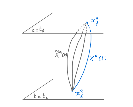
As before, we consider infinitesimal virtual variations \(\delta x^a(t)\). In particular, infinitesimal means that we compute to first order in \(\delta x^a\). Furthermore, recall that such displacements commute with the time derivative, \(\delta \dot x^a(t)=\frac {d}{dt}\delta x^a\).

3.2 Hamilton’s principle

According to d’Alembert’s theorem or principle, natural trajectories satisfy

\begin{equation} \label {eq:138} (m_{(a)}\ddot x_a-F_a)\delta x^a\approx 0. \end{equation}

By an integrations by parts, (which means here using Leibniz rule in the way that is done when doing integrations by parts), we have

\begin{equation} \label {eq:139} \frac {d}{dt}(m_{(a)} \dot x_a\delta x^a)-m_{(a)}\dot x_a\delta \dot x^a-F_a\delta x^a\approx 0. \end{equation}

In terms of the kinetic energy and its variation, we have

\begin{equation} \label {eq:140} T=\frac 12 m_{(a)} \dot x_a\dot x^a,\quad \delta T=m_{(a)}\dot x_a\delta \dot x^a. \end{equation}

The last term on the left hand side of (3.2) is the infinitesimal work done by the applied forces,

\begin{equation} \label {eq:141} \cancel {\delta } W= F_a\delta x^a. \end{equation}

The use of the symbol \(\cancel {\delta }\) is to indicate that in general \(F_a\delta x^a\) is not necessarily integrable and the variation of a single function.

In these terms, D’Alembert’s principle can be written as

\begin{equation} \label {eq:144} \frac {d}{dt}(m_{(a)} \dot x_a\delta x_a)\approx \delta T+\cancel {\delta } W. \end{equation}

When integrating this relation along a natural trajectory, one gets

\begin{equation} \label {eq:145} \Big [m_{(a)} \dot x_a\delta x^a\Big ]^{t_f}_{t_i}\approx \int ^{t_f}_{t_i} dt\, [\delta T+\cancel {\delta } W]. \end{equation}

Limiting oneself to virtual instantaneous variations that do not change the end points, \(\delta x^a(t_i)=0=\delta x^a(t_f)\), we get:

3.3 Least action principle

In the particular case when the forces derive from a potential,

\begin{equation} F_a=-\frac {\partial V}{\partial x^a}\iff F_a\delta x^a=-\delta V. \label {eq:142} \end{equation}

and \(\cancel {\delta } W=-\delta V\). In this case, suitable integrability conditions

\begin{equation} \label {eq:143} \frac {\partial }{\partial x^a} F_b-\frac {\partial }{\partial x^b} F_a=0, \end{equation}

have to be satisfied. The force is conservative and the work does not depend on the path taken between the initial and the end points. We can write (3.7) as

\begin{equation} \label {eq:147} \int ^{t_f}_{t_i} dt\ \delta (T-V)=\delta \int ^{t_f}_{t_i} dt (T-V) \approx 0, \end{equation}

where the variation commutes with integration since it is done at a fixed time. Defining the action, respectively the Lagrangian, as

\begin{equation} \label {eq:148} S[x^a(t)]=\int ^{t_f}_{t_i} dt\ L,\quad L=T-V, \end{equation}

Remarks:

• 1. As in the finite dimensional case considered in the first chapter, where the problem of finding the extrema of a function of several variables, we thus have again an extremisation problem. The analogy is as follows: finding the extrema can be done by finding the points where the gradient vanishes. In the present case this corresponds to solving Newton’s equations. Alternatively, one is looking for the points where the variation of the function vanishes. In the present case, this corresponds to finding the trajectories that extremize the variation of the action. The object whose extremals one is searching for is no longer a function, but a functional, that is to say, the integral of a function \(L\) of several functions \(x^a(t)\) of time. Suppose for instance that \(x^a(t_i)=x^a(t_f)\). One may then develop the trajectories in terms of Fourier series,

  \(\seteqnumber{0}{3.}{12}\)

  \begin{equation} \label {eq:1} x^a(t)=\frac {c_0}{2}+\sum _{n=0}^\infty c^a_n \cos {\frac {2\pi (t-t_i)}{t_f-t_i}}+s^a_n \sin {\frac {2\pi (t-t_i)}{t_f-t_i}}, \end{equation}

  so that, after substitution, the action becomes a function of the Fourier coefficients, \(S[x^a(t)]=S[c_0^a,c_n^a,s_n^a]\) and the extremisation problem becomes that of a function of an infinite, countable number of variables.

• 2. How should one take the constraints into account ? Again there are two options. The first is to explicitly solve the constraints in terms of a number of independent variables \(q^\alpha (t)\) for the trajectories, and reduce the extremisation problem to one in those variables. This is what we will do in detail in the next chapter. The second approach consists in working with Lagrange multipliers, that now also become trajectories, and consider the unconstrained extremisation problem for the extended action

  \(\seteqnumber{0}{3.}{13}\)

  \begin{equation} \label {eq:2a} S[x^a(t),\lambda ^m(t)]=\int _{t_i}^{t_f}dt\ \Big [ L(x^a(t),\dot x^a(t))-\lambda ^m(t) G_m(x^a(t),t)\Big ]. \end{equation}